I went through the last Facebook paper (Carion et al., 2020), which proposes a new architecture, DETR, for object detection and segmentation based on Transformers. To better understand the paper, I decided to review the basic principles of Transformers and Attention. I am not pretending to write the best article on Transformers on the Internet. I just want to reason a bit about Transformers and maybe present the underlying ideas simply and intuitively.
Transformers
Transformers (Vaswani et al., 2017) are a deep learning architecture based on the attention mechanism. They are usually applied to sequential data in NLP tasks. Attention relates different positions of a single sequence in order to compute a meaningful representation of the sequence.
Characteristics:
Attention
The attention function has different inputs in the form of vectors:
- query (denoted as \(q\))
- key-value pairs (denoted as \(k\) and \(v\))
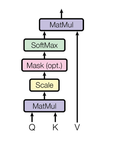
The output is computed as a weighted sum of the values based on the key similarity with respect to the query. It can be described as a retrieval mechanism in which the keys may not be exactly equal to the query. Here, the key similarity is obtained through a compatibility function of the query and the keys.
How to obtain a similarity (or compatibility) score?
This is very easy, you need just to compute the dot product of two vectors. So, let us say you want to compute the similarity of the vectors \(q \in \mathcal{R}^n\) and \(k \in \mathcal{R}^n\):
\[Sim(q, k) = q \cdot k^T .\]If we have one query and multiple keys we can multiply the query vector with all keys arranged in a matrix, denoted as \(K \in \mathcal{R}^{d \times n}\):
\[Sim(q, K) = q \cdot K^T = [Sim(q, k_1), Sim(q, k_2), \dots, Sim(q, k_n)] \in \mathcal{R}^d\]If we have multiple queries and multiple keys we can also arrange the queries in a matrix \(Q \in \mathcal{R}^{m \times n}\):
\[Sim(Q, K) = Q \cdot K^T = \left[ \begin{array}{ccc} Sim(q_1, k_1) & \cdots & Sim(q_1, k_n) \\ \vdots & \ddots & \vdots \\ Sim(q_m, k_1) & \cdots & Sim(q_m, k_n) \end{array} \right]\]Notice that \(Sim(Q, K) \in \mathcal{R}^{m \times d}\).
To understand better the attention as information retrieval mechanism, it is useful to think in these terms.
Let us say we have 3 keys, corresponding to the vectors forming angles of 0, 45 and 90 degrees. Suppose to have a query vector forming an angle of 60 degree. The keys are visualized in blue and the query in red:
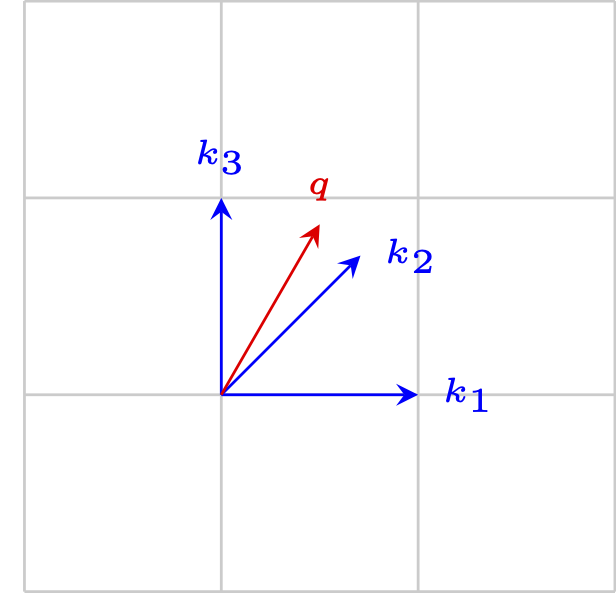
As we can see, the query is similar to keys \(k_2\) and \(k_3\). To quantify the similarity, we calculate the dot product between the query and the keys matrix:
To normalize the similarity matrix, we can apply the \(softmax\) function, obtaining the attention weights:
For larger values of \(n\), query and key dimension, the dot product grows large in magnitude and pushes the softmax (see later) in regions with small gradients. To overcome this limitation, we divide each element of the similarity matrix by \(\sqrt{n}\), the dimension of the query and the key. The attention weights scaled are simply the weights obtained applying the softmax function to the similarity matrix scaled.
Attention Score
Using the softmax we find the weights associated to each value, we can then multiply the weghts by the values obtaining the attention score:
\[\text{Attention}(Q, K, V) = \text{softmax} \left( \frac{QK^T}{\sqrt{n}} \right) V \in \mathcal{R}^{m \times u}\]where \(V \in \mathcal{R}^{d \times u}\).
Going back to our example we can summarize the whole mechanism with the following diagram:

From the query vector and the keys we calculate the attention weights, we can then use the attention weights associated to each key to weight the corresponding value.
Multi-Head Attention
Multi-Head attention refers to the computation of \(h\) attention scores starting from linear projections of the input vectors. These linear projections are learned during training.
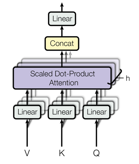
Why Multi-Head Attention?
Using Multi-Head attention the model can exploit different input representations to attend different positions.
Why Linear Projection?
The Linear Projection of the keys and the query is a very important characteristic of the attention mechanism. If we keep the query and key fixed we will end up in learning nothing. A learnable projection is highly fundamental. In this way the input can adapt to the keys and can understand what is important to ask. If we think of the keys as representing attributes of the input sentence, our learned query can ask important attributes for the decoding part.
Self-Attention
In a self-attention layer the keys, values and queries are all the same:
\[\text{Self-Attention}(X) = \text{Attention}(X, X, X)\]Linear Projection in a Self-Attention Layer
In a self-attention layer the linear projection becomes more important. If we compute the self-attention using only the embedding we would only use the similarity defined by the embedding. Using a linear projection we let the embedding to adapt to the specific task. In this way the similarity between inputs can be learned during training. At the same time, learning values can be beneficial as they represent important attributes of the input.
Encoder-Decoder
The Transformer model is made of two parts: an Encoder and a Decoder.
Encoder
The Encoder is a stack of N blocks. Each block is made of two layers:
- Multi-Head (Self-)Attention
- Position-wise Feed Forward Network (FFN)
In addition, the original Transformer uses Residual connections and Layer Normalization.
The Encoder takes the inputs, and it converts it into a latent representation. In the context of NLP, the inputs are the tokenized words projected into an embedding.
A position-wise FFN is a FFN applied to each position in an independent way. Across the same layer, the parameters are shared. This is equivalent to a convolution with kernel size 1.
Decoder
The decoder is a stack of N blocks. Each block is composed of:
- Multi-Head (Self-)Attention considering the outputs
- Multi-Head Attention considering the output of the encoder
- Position-wise FFN
Similarly to the encoder, the decoder uses Residual connections and Layer Normalization.
In a Machine Translation task, the decoder generates token sequentially like an autoregressive model. It starts from the initial token, and it generates a distribution over the next token. The token associated with the highest probability is selected and fed again in the decoder. During this process, the decoder can attend at each position of the output generate up to the current one.
Attention in Transformer
There are three different attention applications in the transformer model:
-
Encoder self-attention. The key, values and queries are the same and comes from the previous layer of the encoder. Motivation: in this way, the encoder can attend to different positions of the previous layer.
-
Encoder-decoder attention. The output of the encoder is used as keys and values, while the queries come from the previous layer of the decoder. This is a very interesting technique. The encoder can suggest interesting keys and values; we can think of them as attributes of the input sequence. The decoder can ask through the query some properties it is interested in. This allows the decoder to attend different positions of the input sequence.
-
Decoder self-attention. The self-attention layer of the decoder allows the encoder to attend all the generated positions up to and including the current position.
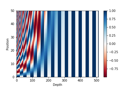
Positional Encoding
The transformer model contains no information about the element position. The inputs are fed into the encoder without keeping the structure in the sentence. Positional-encoding is a rather simple trick to help the network to understand the order of tokens in the sequence. Positional encoding can be learned or fixed.
The paper uses trigonometric functions of different frequencies to encode each position in a differentiable manner:
\[PE(pos, 2i) = \sin \left( \frac{pos}{1e5^{2i/n}} \right) \\ PE(pos, 2i+1) = \cos \left( \frac{pos}{1e5^{2i/n}} \right) ,\]where \(pos\) is the position and \(i\) is the dimension. Each dimension of the positional encoding corresponds to a sinusoid.
It is useful to visualize each dimension of the positional encoding as a sinusoid. The positional encoding of a determined position is the value of all the sinusoids in that position.
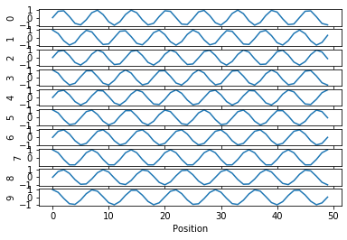
For the sake of visualization, we can arrange the positional encodings in a grid obtaining the following plot:
Transformers vs LSTM
Prior to Transformers, the most used architecture for sequence to sequence learning was the LSTM (Hochreiter & Schmidhuber, 1997). It is beneficial to understand the differences between these two architectures.
Input Handling
LSTM
In an LSTM, the input is analyzed in a sequential fashion, starting from the first token and going on. It is also possible to use a Bidirectional LSTM that analyzes the input from both directions (forward and backward).
Transformer
The transformer processes each input token at the same. Transformers exploit the positional encoding to understand the input structure.
Gradient Flow
LSTM
In an LSTM, the path from an input token to the output depends on the position of the token. The input token goes through a sequence of transformations before being projected in the latent representation. In an LSTM layer, there are \(n\) sequential operations, where \(n\) denotes the sequence length. The number of operations that connects two input positions is proportional to their distance in the sentence.
Transformers
In a Transformer, the path from an input token to the output is shorter, and it does not depend on the input length. This allows transformers to be able to process longer sequences. In an self-attention layer, there is a constant number of sequential operations, not depending on the sequence length. In addition, in a self-attention layer, each input position is connected to the other positions through a single operation.
Output Generation
The output generation of LSTM and Transformer is very similar. Both generate token sequentially, and the current generated token is used to predict the next token.
Other Attention Applications
Self-Attention Generative Adversarial Networks
Self-Attention Generative Adversarial Networks {$ cite Han18 %} employ the Self-Attention mechanism to use global information both in the generator and in the discriminator. GANs are usually based on convolutional building blocks, that
Resources
- Attention is All You Need by Yannic Kilcher
- Transformer model for language understanding, TensorFlow Tutorial
- The Illustrated Transformer by Jay Alammar
References
- [carion2020endtoend] Carion, N., Massa, F., Synnaeve, G., Usunier, N., Kirillov, A., & Zagoruyko, S. (2020). End-to-End Object Detection with Transformers.
- [vaswani_attention_2017] Vaswani, A., Shazeer, N., Parmar, N., Uszkoreit, J., Jones, L., Gomez, A. N., Kaiser, L., & Polosukhin, I. (2017). Attention Is All You Need. ArXiv:1706.03762 [Cs]. http://arxiv.org/abs/1706.03762
- [hochreiter_long_1997] Hochreiter, S., & Schmidhuber, J. (1997). Long Short-Term Memory. Neural Computation, 9(8), 1735–1780. https://doi.org/10.1162/neco.1997.9.8.1735