Object Detection: A Review

In this article, I review some 2D Object Detection papers.

R-CNN

R-CNN (Girshick et al., 2014) (Regions with CNN features) presents a first, preliminary, approach to Object Detection.

Figure 1: R-CNN

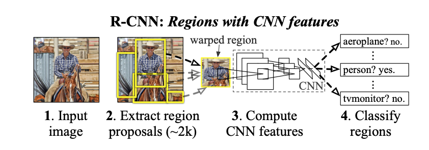
Pipeline:

• Extract around 2000 bottom up region proposals from the input image
• Warp regions to fixed size
• Extract features using a large CNN from warped regions
• Classify each region using class-specific linear SVMs

3 main modules:

• Region proposal:
  Selective search + affine warping to fixed size
• Feature Extraction:
  Extract 4096-dimensional feature vector. Images are “normalized” by subtracting their mean before computing the features
• Image classification

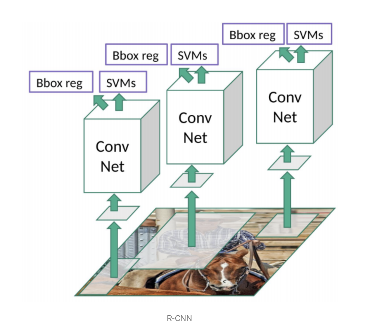
This approach is actually an hand-crafted region proposal followed by a classifier. The standard R-CNN network can be extend with a Bounding Box Regression module to improve localization performance.

After scoring each proposal with a class-specific SVM, a class-specific bounding-box regressor is applied to the CNN features.

The bounding box regression module predicts 4 parameters, \(d_x, d_y, d_w, d_h\) such that, given the proposal bounding box \(P_x, P_y, P_w, P_h\), the final box is predicted as:

\[G_x = P_w d_x + P_x \\ G_y = P_h d_y + P_y \\ G_w = P_w exp(d_w)\\ G_h = P_h exp(d_h)\]

In words, the module predicts:

• A shift (\(d_x\), \(d_y\)) that is relative to the bounding box width and height
• The log of ratio between the real size and the proposal size. If the ratio is 1, the proposal size is equal to the ground truth size and the network can just predict 0. If the real height is smaller than the proposal height, the network should predict \(d_h < 0\), otherwise \(d_h > 0\). The same reasoning applies to the proposal width.

The authors do not actually learn the parameters of the network, they solve the problem in closed form using regularized least squares.

Figure 2 shows the final architecture of R-CNN.

Figure 2: Full architecture of R-CNN

Problems:

• Huge amount of time to train the network for each of the 2000 proposals regardless of the content of the image
• Not real time, inference around 47 seconds
• Selective search is a hand-crafted algorithm, no learning involved.

Fast R-CNN

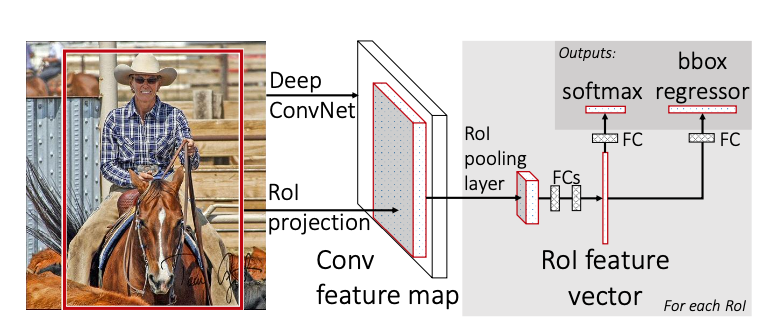
Fast R-CNN (Girshick, 2015), from the same authors of R-CNN, represents an improvement over the previous architecture. As in R-CNN, in Fast R-CNN the Network takes as input a set of RoIs (no learning is involved in this stage). Differently from R-CNN, the CNN backbone processes the whole image to extract features. Each RoI is pooled (through RoI Pooling) into a fixed-size feature map. The feature map is flattened and feeded into Fully Connected layers. The Network outputs softmax scores and bounding box parameters for each RoI.

Figure 3: Fast R-CNN architecture.

Key ideas and contributions (my opinion):

• RoI (max) Pooling
• Smooth L1 Loss for localization
• Truncated SVD for fully connected layers for performance reasons

Main pipeline:

• Hand-crafted RoIs from input image
• The CNN backbone processes the whole image (differently from R-CNN)
• RoI Pooling to obtain fixed size images from input RoI and CNN features
• Fully Connected layers to obtain class scores and bounding box refinement

RoI Pooling

RoI Pooling, or RoI Max Pooling, maps the input RoI into a fixed size feature map. The output map has a fixed dimension of \(H \times W\), hyperparameters independent with respect to the RoI.

How does it work?

Let’s say the input RoI has a size of \(h \times w\). RoI Pooling divides the RoI into sub-regions of size \(h/W \times w/W\). Max-Pooling is applied into sub-regions to obtain the output value for the sub-region.

Figure 4: Roi Pooling.
Credit: deepsense.ai

Back-propagation through RoI Pooling.

RoI pooling is mathematically non-differentiable as it involves the max function for each region. The approximated derivative is back-propagated only through the value corresponding to the max of each region, with the assumption that a small perturbation of the input would not change the maximum value.

Loss

Fast-RCNN uses a Smooth \(L_1\) loss for localization, less sensitive to outliers than the standard \(L_2\) loss.

\[L_{\text{loc}} = \sum_{i \in {x, y, w, h}} \text{smooth}_{L_1} (p_i - g_i),\]

where

\[\text{smooth}_{L_1}(x) = \begin{cases} 0.5 x^2 & \text{if} |x| < 1 \\ |x| - 0.5 & \text{otherwise}. \end{cases}\]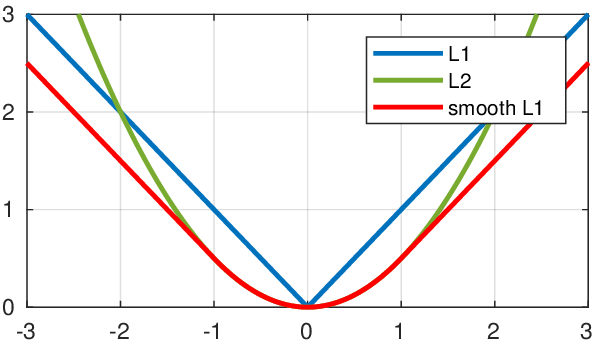

Faster R-CNN

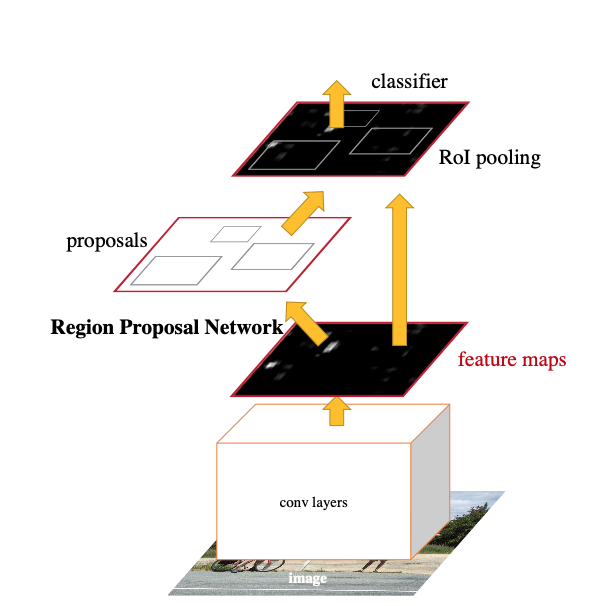
Faster R-CNN (Ren et al., 2016), again from the same authors, tries to solve the region proposal problem of the previous approaches. In the previous approaches, region proposal was an hand-crafted and time expensive algorithm, with no learning involved. At that time the two SOTA methods for region proposals were Selective Search and EdgeBoxes. Selective Search took 2 seconds per image in a CPU implementation. EdgeBoxes took 0.2 seconds per image, was the best tradeoff between proposal quality and speed.

Faster R-CNN focuses on computing proposals with a deep convolutional network to share computation between the proposal task and the detection task. Given the feature maps extracted from the backbone, the RPN (Region Proposal Network) extracts region proposals, that are used as input for the detection network, together with the convolutional features.

Figure 5: Faster R-CNN architecture

Key ideas and contributions (my opinion):

• Region Proposal Networks
• Anchor concept
• Feature sharing between region proposals and object detection

Region Proposal Networks

The Region Proposal Network takes as input the output of the backbone network. A \(n \times n\) convolutional layer is followed by two \(1 \times 1\) convolutional layers, predicting the class and the bounding box parameters. At each sliding window location, multiple proposals are predicted simultaneously, we denote with \(k\) the number of proposals.

The regression layer has \(4\) outputs for each proposal encoding the parameters of the \(k\) boxes, so in total \(4k\) outputs. The \(k\) proposals are parameterized with respect to \(k\) reference boxes, called anchors. Each anchors is centered in the considered region and associated with a specific scale and aspect ratio. The authors used 9 anchors at each location.

The class prediction layer has 2 outputs for each proposal, the probability of object and the probability of background (no object), so in total \(2k\) outputs.

Loss

In order to train the RPN to predict the objectness score for each anchor, we must assign the ground truth label to each anchor.

• Positive label:
  • IoU higher than a threshold (0.7) with any ground truth box
  • Highest IoU overlap with a given ground truth box, even if less than threshold
• Negative label:
  • IoU lower than th (0.3) for all ground truth boxes.
• Don’t care label:
  • Anchors that are neither positive or negative do not contribute to the loss

Given the label for each anchor, a simple classification loss is used.

Mask R-CNN

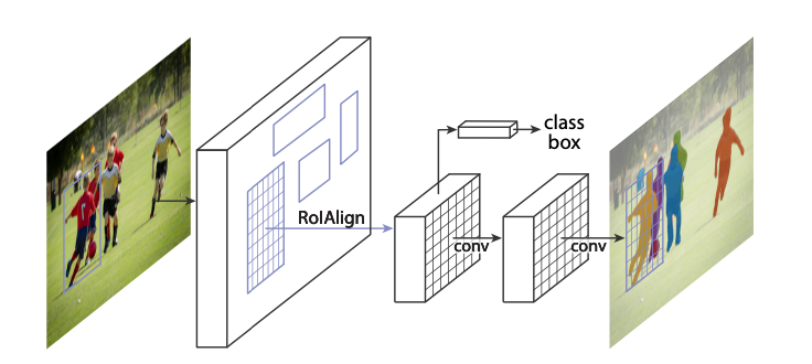
Mask R-CNN (He et al., 2018) extends Faster R-CNN adding an object mask branch in parallel to the class prediction and box prediction branches. The goal of the network is to perform instance segmentation, identifying for each object in the image the associated pixels. Notice: this is different from semantic segmentation whose goal is to correctly classify pixels in a fixed set of categories without differentiating between object instances.

The main problem when trying to extend Faster R-CNN for instance segmentation tasks is that it was not designed for pixel to pixel alignment between inputs and outputs. This is due mainly to the Roi Pooling layer, that performs coarse spatial quantization. For this reason, Mask R-CNN introduces Roi Align layer that preserves exact spatial locations.

An interesting feature of Mask R-CNN is that the mask prediction is performed independently for each class. At inference time, the mask corresponding to the predicted class is used combining in this way class prediction and mask prediction without competition among classes.

Figure 6: Mask R-CNN architecture

Mask Prediction

The mask branch outputs \(K\) binary masks of resolution \(m \times m\), one for each of the \(K\) classes. At the end, no softmax is applied, as it is usually done for semantic segmentation tasks. A per-pixel sigmoid activation is applied to scale the score of each mask in the range (0, 1). The mask loss is calculated only for the ground truth mask, while the other masks do not contribute to the loss. In this way, a mask is generate for every class without competition among classes and the output mask is selected by the class prediction layer. This effectively decouples mask and class prediction.

RoI Align

Let’s see the problems of RoI Pooling before exploring the RoI Align layer. RoI pooling first quantizes the proposed RoI to the granularity of the feature map. The quantized RoI is divided into spatial bins, again quantixed. For each bin, values are aggregated through max pooling. This has a negative effect on the prediction of pixel-accurate segmentation masks, while the classification and detection tasks are usually robust with respect to small translations.

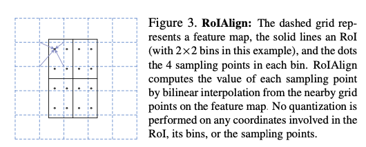
RoI Align tries to properly align the extracted features with the input. Given the input RoI, no quantization is applied. The RoI is then divided into bins, for each bin four regularly sampled locations are used to calculate the values of input features through bilinear sampling.

Figure 7: RoI Align

Focus: Bi-Linear Interpolation

Bi-Linear interpolation applies linear interpolation in two directions. It uses 4 nearest neighbors to output the final value of the interpolated point.

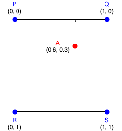
Suppose we want to perform bi-linear interpolation using the query point A (0.6, 0.3) in this situation:

Figure 8: Bi-Linear 1

Bi-Linear interpolation performs a first linear interpolation for the two rows finding the values of the locations B(0.6, 0) and C(0.6, 1).

Figure 9: Bi-Linear 2

\[\color{green}{B} = \frac{A_x - P_x}{Q_x - P_x} \color{blue}{P} + \frac{Q_x - A_x}{Q_x - P_x} \color{blue}{Q} \\ \color{green}{C} = \frac{A_x - R_x}{S_x - R_x} \color{blue}{R} + \frac{S_x - A_x}{S_x - R_x} \color{blue}{S} \\\]

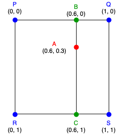
Then, the final value is another linear interpolation between the values B and C considering only the y-coordinate:

\[\color{red}{A} = \frac{A_y - B_y}{C_y - B_y} \color{green}{B} + \frac{C_y - A_y}{C_y - B_y} \color{green}{C}\]

Extra: Tri-Linear interpolation At this point it is interesting to see how bilinear interpolation extends to 3 dimension. This is not actually linked to RoI Align, but it is still interesting. Tri-Linear interpolation can be seen as a linear interpolation of two bi-linear interpolation.

Figure 10: Tri-Linear Interpolation

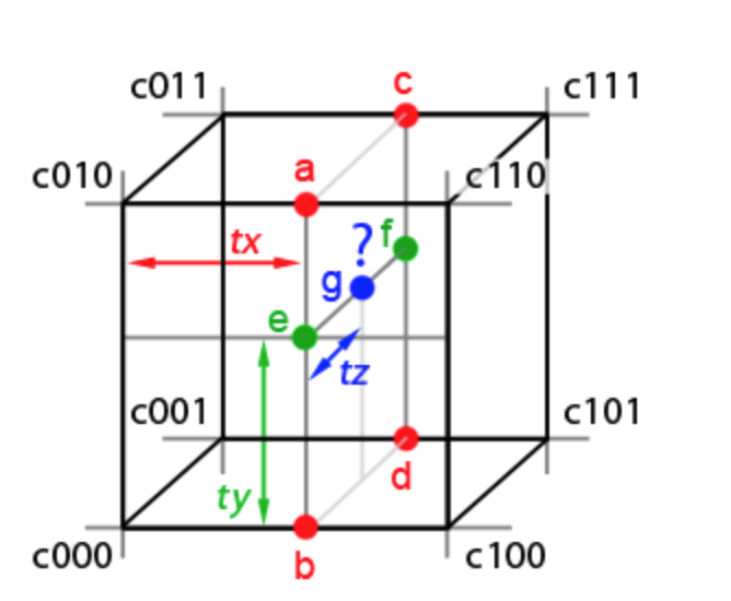
Given the query point g, we first compute the values a b c d using the quantity tx. We then compute e f interpolating a b c d using ty and finally we find the value of the query point g interpolating e f through tz.

References

1. [rcnn_2014] Girshick, R., Donahue, J., Darrell, T., & Malik, J. (2014). Rich feature hierarchies for accurate object detection and semantic segmentation.
2. [fastrcnn_2015] Girshick, R. (2015). Fast R-CNN.
3. [faster_rcnn_2016] Ren, S., He, K., Girshick, R., & Sun, J. (2016). Faster R-CNN: Towards Real-Time Object Detection with Region Proposal Networks.
4. [mask_rcnn_2018] He, K., Gkioxari, G., Dollár, P., & Girshick, R. (2018). Mask R-CNN.