In this article we present our approach for the NIPS 2017 ”Learning To Run” challenge. The goal of the challenge is to develop a controller able to run in a complex environment, by training a model with Deep Reinforcement Learning methods. We follow the approach of the team Reason8 (3rd place). We begin from the algorithm that performed better on the task, Deep Deterministic Policy Gradient (DDPG). We implement and benchmark several improvements over vanilla DDPG, including parallel sampling, parameter noise, layer normalization and domain specific changes. We were able to reproduce results of the Reason8 team, obtaining a model able to run for more than 30m.
Background
Reinforcement Learning (RL) deals with sequential descision making problems. At each time step the agent observes the world state, selects an action and receives a reward.
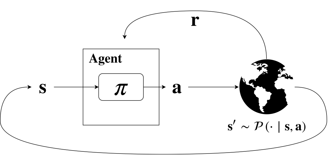
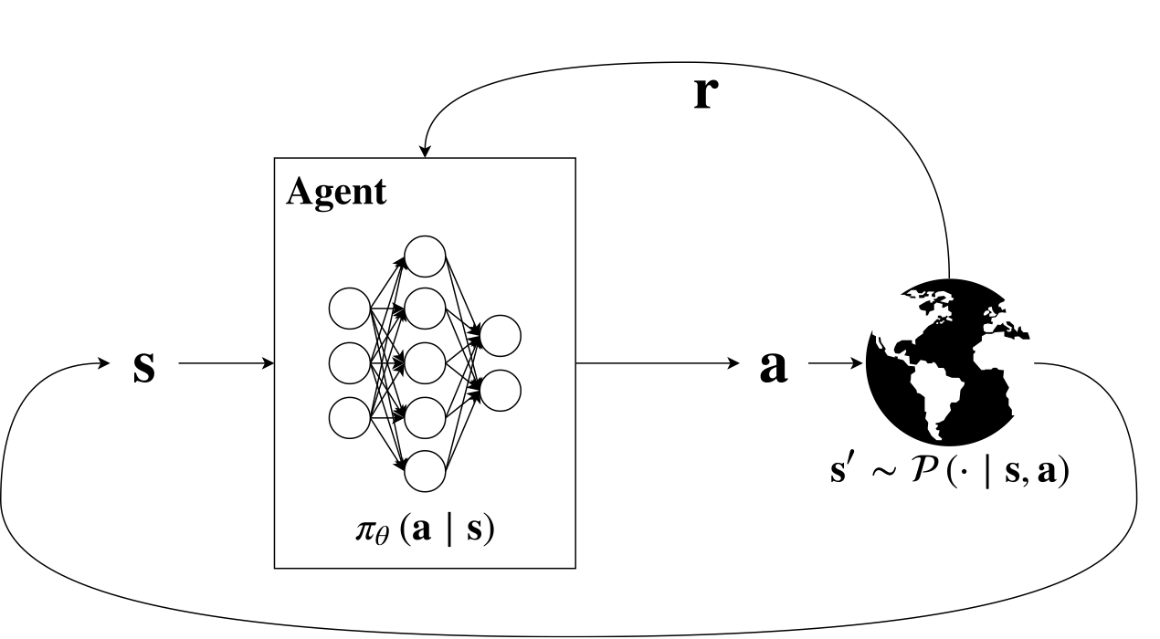
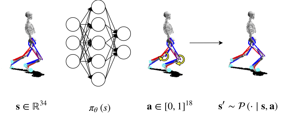
The figure above represents the Reinforcement Learning framework. The agent receives, at each time step a representation \( s \) of the state of the system. The agent takes an action a, according to its policy \( \pi \). The action has an effect on the world. The effect is a transition to the state \( s’ \), according to the world dynamic \( P \). At the same time the agent receives a reward \( r \), based on the action and on the state. The policy \( \pi \) is often encoded in a neural network.
The RL goal is to maximize the expected discounted sum of rewards:
\[J_\pi = \mathbb{E}\left[\sum_{t=0}^H \gamma^t r(s_t,a_t) \right] \, .\]Where \( J \) represents the objective function, \( \gamma \) is the discount factor, \( r \) is the reward and \( H \) is the horizon length.
How can we achieve this goal?
Gradient ascent over policy parameters:
\[\theta' = \theta + \eta \nabla_\theta J_\pi .\]Where the update of the policy parameters \( \theta \) follows the gradient of the objective function \( \nabla J \). A straightforward approach to accomplish this is presented in (Williams, 1992) with REINFORCE algorithm, that uses Monte Carlo sampling to estimate the performance gradient considering a stochastic policy. Deterministic Policy Gradient (DPG) (Silver et al., 2014) expands on this by considering deterministic policies only, for continuous action spaces. To ensure adequate exploration, an off-policy actor-critic algorithm is introduced to learn a deterministic target policy from an exploratory behavior policy. However, directly using neural networks as function approximators leads to unsatisfactory results due to two problems:
- most optimization algorithms for neural networks assume that samples are independently and identically distributed, which is not true when samples are generated from exploring sequentially in an environment;
- since the network Q, part of Q-learning algorithms, being updated is also used in calculating the target value, the Q update is prone to divergence.
DQN (Mnih et al., 2013) implements Q-learning using a deep neural network to approximate the Q function. To address the problem (1.) DQN introduces a replay buffer which stores transitions generated by the environment. During training, a batch of transitions is drawn from the buffer to restore the i.i.d. property. Although, since a maximization over the action space is required, DQN does not scale with high-dimensional and continuous action spaces. Deep Deterministic Policy Gradient (DDPG) (Lillicrap et al., 2016) solves all the these problems by using:
- A deterministic parametrization of the actor \( \pi \), updated in the direction of the gradient of \( Q(s, \pi(s)) \). This is a scalable alternative to global maximization, that is infeasible in high-dimensional continuous action spaces;
- A replay buffer;
- Separated target networks with soft-updates to improve convergence stability.
Deep Deterministic Policy Gradient
DDPG is a state of the art algorithm in Deep Reinforcement Learning.
Off policy
DDPG is an off-policy method, which means that the optimized policy is different from the behavioral policy. Off-policy algorithm usually allow re-usage of all the samples, whereas on-policy approaches would require to throw them away at each update.
Actor Critic
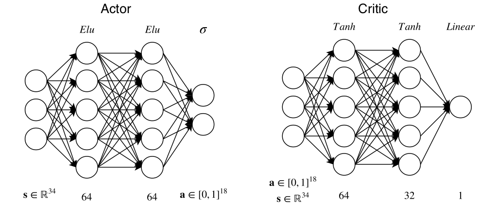
Actor critic algorithm uses two networks. The actor network represents the agent policy and outputs an action given a state. The critic network takes as input the pair state action and outputs an estimates of the quality of the action in that state. The two networks used in our project are the followings:
Critic is trained using off-policy data coming from the replay buffer, that is a FIFO queue containing tuples \( (s_t, a_t, r_t, s_{t+1}) \). Critic’s task is to minimize the Bellman error (notice that the policy is deterministic, so we can avoid the expectation over actions):
\[Q(s_t,a_t \mid \theta^Q ) = r(s_t,a_t) + \gamma Q(s_{t+1}, \pi (s_{t+1} \mid \theta^\pi ) \mid \theta^Q ),\]where \( \theta^Q \) are parameters of the critic network and \( \theta^\pi \) are actor’s parameters. It is evident in the equation above that the update step of the weights \( \theta^Q \) comprises \( Q(s_t, a_t \mid \theta^Q) \) in the target, resulting in an iterative update prone to divergence. DDPG solves this problem using target networks. Target networks are copies of the actor and critic networks that are only used for computing target values, and softly updated for improving stability:
\[\theta' = \tau \theta + (1-\tau)\theta' \qquad \tau \ll 1,\]where \( \theta \) are the weights of the original network and \( \theta’ \) the weights of the target networks.
The resulting error for the critic network is:
\[L = \frac{1}{N} \sum_{i=1}^N (y_i - Q(s_i, a_i \mid \theta^Q))^2 \, ,\]with target:
\[y_i = r_i + \gamma Q(s_i, \pi(s_i \mid \theta'^\pi) \mid \theta'^{Q}).\]The actor is updated using the estimated deterministic policy gradient, here reported for the sake of completeness:
\[\nabla_{\theta^\pi}J \approx \frac{1}{N} \sum_{i=1}^N \nabla_a Q(s, a \mid \theta^Q) \mid_{s = s_i, a = \pi(s_i)} \nabla_{\theta^\pi} \pi(s \mid \theta^\pi)\mid_{s_i}.\]Applying the vanilla DDPG algorithm to the learning to run task leads to unsatisfactory results as we can see from the initial video.
DDPG Improvements
Parallel Sampling
A key step in any reinforcement learning algorithm is the generation of \( (s_t, a_t, r_t, s_{t+1}) \) transitions to gather information from the environment. Since our simulator is very slow, making this step as fast as possible is desirable. Parallelization in our algorithm is implemented through three types of threads: sampling threads, training thread and evaluation threads. Each sampling thread is tasked with collecting trajectories using the provided policy, pushing them in a common queue and waiting for a new policy.
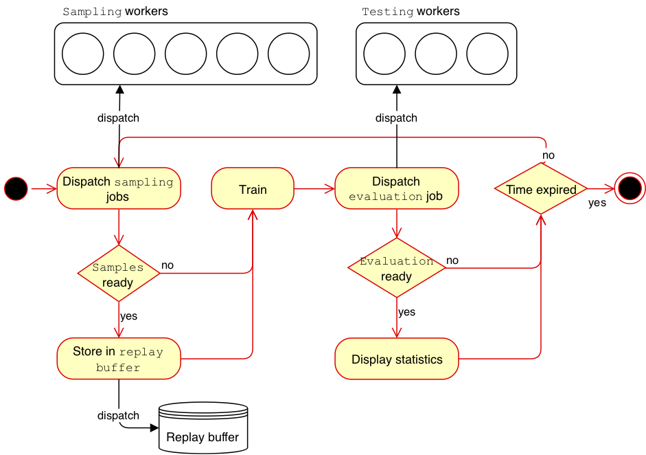
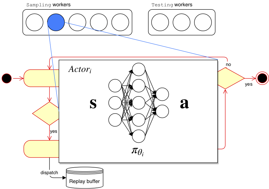
The training thread waits samples from \( m \) sampling threads, stores them in the replay buffer and trains the actor and critic networks for a fixed number of training steps. The new actor network is then sent to the waiting sampling threads that can now restart the sampling process. Evaluation threads are spawned every fixed number of training steps. Having multiple sampling threads running policies with different weights improves exploration and results in a substantial performance improvement. We used 20 sampling threads, 1 training thread and 5 evaluation threads in our implementation. We found out in our experiments that \( m=1 \) is a good trade-off between sampling and training.
Exploration
To explore we used action noise and parameter noise (Plappert et al., 2017) in an alternated way. At the beginning of an episode we selected between action noise and parameter noise with 0.7 and 0.3 probability respectively. Action noise is directly applied to the action selected by the actor network. We used an Ornstein-Uhlenbeck (OU) (Uhlenbeck & Ornstein, 1930) process to generate correlated noise for efficient exploration in physics based environments. Parameter noise perturbs actor network weights to obtain a state dependent exploration, thus more coherent with respect to action noise. The noise used in parameter noise is sampled at the beginning of an episode and it’s kept fixed for all the episode. Parameter noise works well with layer normalization (Ba et al., 2016). Layer normalization, as the name says, normalizes the output of a selected layer. This technique, besides stabilizing training, makes possible to use the same perturbation scale across all network layers. We used layer normalization both for actor and critic networks applying it to all layer except the last one before the non linearity.
States and actions flip
The model has a symmetric body, thus it’s easy to increase the sample size by flipping states and actions. Flipping a state means to swap left and right parts of the body, flipping an action means to swap actuations of left and right legs. States and actions flip is implemented in this way: we sample transitions \( (s_t, a_t, r_t, s_{t+1}) \) from the replay buffer, flip state components of \( s_t \) and \( s_{t+1} \), flip the action \( a_t \) and add to the batch original as well as flipped transition. This has an easy interpretation: we know that if action \( a_t \) in state \( s_t \) , results in state \( s_{t+1} \) and in a reward signal \( r_t \), doing the symmetric action with respect to \( a_t\) in the symmetric state with respect to \( s_t \) results in the symmetric state with respect to \( s_{t+1} \) and in the same reward signal \( r_t \). Flipping transitions helps in obtaining symmetric policies, that is desirable since running is a symmetric task.
Environment
The agent is a musculoskeletal model including information about muscles, joints and links moving in a 2D environment (no movement is possible along Z axis).
Kinematic quantities are provided for body parts and joints, while activation, fiber length and fiber velocity are provided for muscles.
The total amount of variables describing the state of the agent is 146.
The agent can actuate 9 muscles for each leg, thus \( a \in [0,1]^{18} \).
In our version of the environment we removed obstacles, obtaining a slightly easier version of the task.
Reward is defined as the change in the x coordinate of the pelvis for each step plus a small penalty for using ligament forces.
An episode terminates when the agent falls (pelvis \( y < 0.65 \)) or after 1000 steps.
Simulation is based on the OpenSim library that relies on the SimBody physics engine. Due to a complex physics engine the environment is quite slow compared to standard RL environments (Roboschool, Mojoco, etc.) and a step can take seconds, thus it is crucial to use the most sample-efficient method.
Environment modifications
We used several modifications of the environment during training to improve efficiency and to help the learning algorithm.
Reward
We added a small bonus to the reward for each time-step survived. We did not study the contribution of this change thoroughly, but we expect it to add some greediness to the initial training steps to favor policies that keeps the model standing.
Environment accuracy
We used a lower integrator accuracy with respect to the standard one of the simulator obtaining 5x speedup. After some episodes the environment becomes slower with respect to initial episodes, probably for a memory leak. We solved this problem doing a reset of the environment after 100 episodes.
Relative positions
As mentioned above, position vectors of the model body parts are exposed by the simulator as absolute. For the purpose of learning, keeping an absolute reference frame is undesirable. In fact, being running an approximately periodic task, having the skeleton in some position at a given distance from the origin, should make no difference from having it in the same position at another distance. Therefore, we modified the observation vector by centering the \( x \) coordinates of the body parts around the pelvis \( x \). Exploiting such symmetry of the model enables shorter learning time and, most importantly, higher generalization.
State variables
OpenSim exposes a number of variables for a musculoskeletal model. Even though to preserve the Markovian property we should consider them all, many of them are in practice useless for the task to learn. In training our model, two subsets of them were considered and we refer to them as full-state and reduced-state. Reduced-state comprises the \( x \), \( y\) position of body parts, the rotation and rotational speed of joints, the speed and position of the center of mass, resulting in \( s \in \mathbb{R}^{34}\). Namely body parts are head, torso, right and left toes and talus and joints are ground pelvis and left and right ankles, hips and knees. Full-state takes into account all the variables from reduced-state, together with the speed and acceleration of body parts and acceleration of joints, resulting in \( s \in \mathbb{R}^{67} \).
Results
For all the experiments we ran DDPG algorithm with the modifications we describe in sections DDPG improvements and Environment modifications. We performed an ablation study to test the relevance of our main changes to vanilla implementation. We compared the performance of a model trained on the reduced-state space with respect to the full-state space. Moreover we compared the quality of the models learned with or without state-action-flip and parameter noise, in terms of performance and required training steps. All the models running on the reduced-state configuration share the same architecture for actor and critic networks, with Xavier initialization (Glorot & Bengio, 2010) for the neurons.
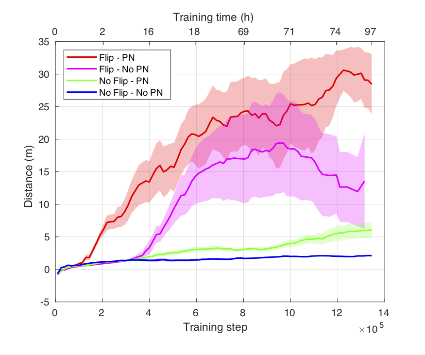
State action flip and parameter noise
In this experiment we investigated on the importance of state-action flip and parameter noise (PN) for the learning process. We trained four models for approximately \( 10^6 \) training steps with all the combinations of the two improvements, i.e. with and without state-action flip and parameter noise. From our experimental results, introducing both modifications leads to both better performance, in terms of longer run distance, and a significant speed-up in terms of training steps to reach same distance. It is also worth highlighting that the learned model with state-action flip achieved higher performance than the one with PN only. This possibly remarks the importance of domain-specific additions in the context of RL which outperformed an uninformed exploration.
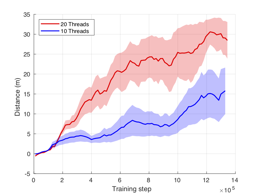
Sampling threads
In this experiment we analyzed the impact of the number of sampling threads. We trained two models with 10 and 20 sampling threads respectively. We used the same sampling-training strategy: wait for samples from 1 thread, check the state of the other threads (collecting samples if available), train for 300 steps, send the updated policies to waiting threads that restart the sampling process. The experiment with 20 sampling threads outperformed the experiment with 10 sampling threads. This shows the importance of exploration in this task, as well as the importance of parallelization.
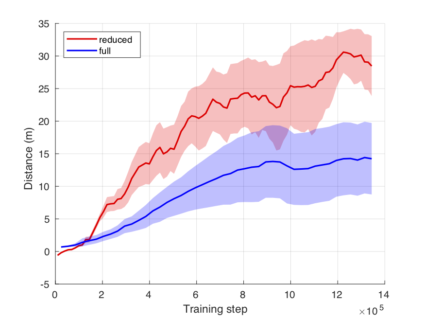
Full vs Reduced state
In this experiment we compared the performance of two learned models, the first trained over full-state space and the second over reduced-state space. The former was trained using a \( [150, 64] \) elu actor network and a \( [150, 50]\) tanh critic network. The latter was trained with a \( [64, 64] \) elu actor network and a \( [64, 32] \) tanh critic network. From our experiments, models trained with a reduce-state space outperformed those trained with the bigger state space. Full-state space introduces several variables that could help in learning a controller for our task, but they also increase the complexity of the model. We did not test thoroughly the networks architecture for the full-state space and incrementing the number of neurons might lead to better performance.
Authors
- Emanuele Ghelfi
- Leonardo Arcari
- Emiliano Gagliardi
References
- [Williams1992] Williams, R. J. (1992). Simple statistical gradient-following algorithms for connectionist reinforcement learning. Machine Learning, 8(3), 229–256. https://doi.org/10.1007/BF00992696
- [dpg] Silver et al., D. (2014). Deterministic Policy Gradient Algorithms. ICML.
- [dqn] Mnih, V., Kavukcuoglu, K., Silver, D., Graves, A., Antonoglou, I., Wierstra, D., & Riedmiller, M. (2013). Playing Atari with Deep Reinforcement Learning. ArXiv:1312.5602 [Cs]. http://arxiv.org/abs/1312.5602
- [ddpg] Lillicrap et al., T. P. (2016). Continuous control with deep reinforcement learning. https://arxiv.org/abs/1509.02971
- [param_noise] Plappert, M., Houthooft, R., Dhariwal, P., Sidor, S., Chen, R. Y., Chen, X., Asfour, T., Abbeel, P., & Andrychowicz, M. (2017). Parameter Space Noise for Exploration. CoRR, abs/1706.01905. http://arxiv.org/abs/1706.01905
- [ou_noise] Uhlenbeck, G. E., & Ornstein, L. S. (1930). On the Theory of the Brownian Motion. Phys. Rev., 36(5), 823–841. https://doi.org/10.1103/PhysRev.36.823
- [layer_normalization] Ba, J. L., Kiros, J. R., & Hinton, G. E. (2016). Layer Normalization. ArXiv:1607.06450 [Cs, Stat]. http://arxiv.org/abs/1607.06450
- [pmlr-v9-glorot10a] Glorot, X., & Bengio, Y. (2010). Understanding the difficulty of training deep feedforward neural networks. In Y. W. Teh & M. Titterington (Eds.), Proceedings of the Thirteenth International Conference on Artificial Intelligence and Statistics (Vol. 9, pp. 249–256). PMLR. http://proceedings.mlr.press/v9/glorot10a.html